Riemann zeta function

The Riemann zeta function Template:Math plotted with domain coloring.

The pole at $z=1$ and two zeros on the critical line.

The Riemann zeta function or Euler–Riemann zeta function, denoted by the Greek letter Template:Math (zeta), is a mathematical function of a complex variable defined as $$\zeta (s)=\sum _{n=1}^{\mathrm{\infty }}\frac{1}{n^s}=\frac{1}{1^s}+\frac{1}{2^s}+\frac{1}{3^s}+\cdots$$ for Template:Nowrap and its analytic continuation elsewhere.

The Riemann zeta function plays a pivotal role in analytic number theory and has applications in physics, probability theory, and applied statistics.

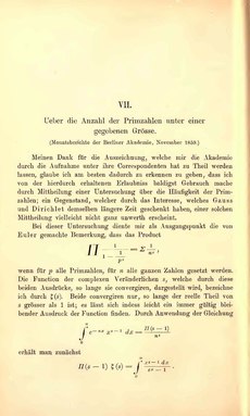
Leonhard Euler first introduced and studied the function over the reals in the first half of the eighteenth century. Bernhard Riemann's 1859 article "On the Number of Primes Less Than a Given Magnitude" extended the Euler definition to a complex variable, proved its meromorphic continuation and functional equation, and established a relation between its zeros and the distribution of prime numbers. This paper also contained the Riemann hypothesis, a conjecture about the distribution of complex zeros of the Riemann zeta function that many mathematicians consider the most important unsolved problem in pure mathematics.

The values of the Riemann zeta function at even positive integers were computed by Euler. The first of them, Template:Math, provides a solution to the Basel problem. In 1979 Roger Apéry proved the irrationality of Template:Math. The values at negative integer points, also found by Euler, are rational numbers and play an important role in the theory of modular forms. Many generalizations of the Riemann zeta function, such as Dirichlet series, [[Dirichlet L-function|Dirichlet Template:Mvar-functions]] and [[L-function|Template:Mvar-functions]], are known.

Definition

Bernhard Riemann's article On the number of primes below a given magnitude

The Riemann zeta function Template:Math is a function of a complex variable Template:Math, where Template:Mvar and Template:Mvar are real numbers. (The notation Template:Mvar, Template:Mvar, and Template:Mvar is used traditionally in the study of the zeta function, following Riemann.) When Template:Math, the function can be written as a converging summation or as an integral:

$\zeta (s)=\sum _{n=1}^{\mathrm{\infty }}\frac{1}{n^s}=\frac{1}{\mathrm{\Gamma }(s)}\underset{0}{\overset{\mathrm{\infty }}{\int }}\frac{x^{s-1}}{e^x-1}\mathrm{d}x,$

where

$\mathrm{\Gamma }(s)=\underset{0}{\overset{\mathrm{\infty }}{\int }}{x}^{s-1}{e}^{-x}\mathrm{d}x$

is the gamma function. The Riemann zeta function is defined for other complex values via analytic continuation of the function defined for Template:Math.

Leonhard Euler considered the above series in 1740 for positive integer values of Template:Mvar, and later Chebyshev extended the definition to $\mathrm{Re}(s)>1.$

The above series is a prototypical Dirichlet series that converges absolutely to an analytic function for Template:Mvar such that Template:Math and diverges for all other values of Template:Mvar. Riemann showed that the function defined by the series on the half-plane of convergence can be continued analytically to all complex values Template:Math. For Template:Math, the series is the harmonic series which diverges to Template:Math, and $$\underset{s\to 1}{\lim }(s-1)\zeta (s)=1.$$ Thus the Riemann zeta function is a meromorphic function on the whole complex plane, which is holomorphic everywhere except for a simple pole at Template:Math with residue Template:Math.

Euler's product formula

In 1737, the connection between the zeta function and prime numbers was discovered by Euler, who proved the identity

$\sum _{n=1}^{\mathrm{\infty }}\frac{1}{n^s}=\prod _{p\text{ prime}}\frac{1}{1-p^{-s}},$

where, by definition, the left hand side is Template:Math and the infinite product on the right hand side extends over all prime numbers Template:Mvar (such expressions are called Euler products):

$\prod _{p\text{ prime}}\frac{1}{1-p^{-s}}=\frac{1}{1-2^{-s}}\cdot \frac{1}{1-3^{-s}}\cdot \frac{1}{1-5^{-s}}\cdot \frac{1}{1-7^{-s}}\cdot \frac{1}{1-11^{-s}}\cdots \frac{1}{1-p^{-s}}\cdots$

Both sides of the Euler product formula converge for Template:Math. The proof of Euler's identity uses only the formula for the geometric series and the fundamental theorem of arithmetic. Since the harmonic series, obtained when Template:Math, diverges, Euler's formula (which becomes Template:Math) implies that there are infinitely many primes. Since the logarithm of Template:Math is approximately Template:Math, the formula can also be used to prove the stronger result that the sum of the reciprocals of the primes is infinite. On the other hand, combining that with the sieve of Eratosthenes shows that the density of the set of primes within the set of positive integers is zero.

The Euler product formula can be used to calculate the asymptotic probability that Template:Mvar randomly selected integers are set-wise coprime. Intuitively, the probability that any single number is divisible by a prime (or any integer) Template:Mvar is Template:Math. Hence the probability that Template:Mvar numbers are all divisible by this prime is Template:Math, and the probability that at least one of them is not is Template:Math. Now, for distinct primes, these divisibility events are mutually independent because the candidate divisors are coprime (a number is divisible by coprime divisors Template:Mvar and Template:Mvar if and only if it is divisible by Template:Mvar, an event which occurs with probability Template:Math). Thus the asymptotic probability that Template:Mvar numbers are coprime is given by a product over all primes,

$\prod _{p\text{ prime}}(1-\frac{1}{p^s})={\left(\prod _{p\text{ prime}}\frac{1}{1-p^{-s}}\right)}^{-1}=\frac{1}{\zeta (s)}.$

Riemann's functional equation

This zeta function satisfies the functional equation $$\zeta (s)=2^s{\pi }^{s-1}\sin \left(\frac{\pi s}{2}\right)\mathrm{\Gamma }(1-s)\zeta (1-s),$$ where Template:Math is the gamma function. This is an equality of meromorphic functions valid on the whole complex plane. The equation relates values of the Riemann zeta function at the points Template:Mvar and Template:Math, in particular relating even positive integers with odd negative integers. Owing to the zeros of the sine function, the functional equation implies that Template:Math has a simple zero at each even negative integer Template:Math, known as the trivial zeros of Template:Math. When Template:Mvar is an even positive integer, the product Template:Nobr on the right is non-zero because Template:Math has a simple pole, which cancels the simple zero of the sine factor.

The functional equation was established by Riemann in his 1859 paper "On the Number of Primes Less Than a Given Magnitude" and used to construct the analytic continuation in the first place.

Equivalencies

An equivalent relationship had been conjectured by Euler over a hundred years earlier, in 1749, for the Dirichlet eta function (the alternating zeta function): $$\eta (s)=\sum _{n=1}^{\mathrm{\infty }}\frac{(-1{)}^{n+1}}{n^s}=(1-2^{1-s})\zeta (s).$$

Incidentally, this relation gives an equation for calculating Template:Math in the region Template:Nobr i.e. $$\zeta (s)=\frac{1}{1-2^{1-s}}\sum _{n=1}^{\mathrm{\infty }}\frac{(-1{)}^{n+1}}{n^s}$$ where the η-series is convergent (albeit non-absolutely) in the larger half-plane Template:Math (for a more detailed survey on the history of the functional equation, see e.g. Blagouchine).

Riemann also found a symmetric version of the functional equation applying to the Template:Math-function: $$\xi (s)=\frac{1}{2}{\pi }^{-\frac{s}{2}}s(s-1)\mathrm{\Gamma }\left(\frac{s}{2}\right)\zeta (s),$$ which satisfies: $$\xi (s)=\xi (1-s).$$

(Riemann's [[Riemann Ξ function|original Template:Math]] was slightly different.)

The ${\pi }^{-s/2}\mathrm{\Gamma }(s/2)$ factor was not well-understood at the time of Riemann, until John Tate's (1950) thesis, in which it was shown that this so-called "Gamma factor" is in fact the local L-factor corresponding to the Archimedean place, the other factors in the Euler product expansion being the local L-factors of the non-Archimedean places.

Zeros, the critical line, and the Riemann hypothesis

Riemann zeta spiral along the critical line from height 999000 to a million (from red to violet)

The Riemann zeta function has no zeros to the right of Template:Math or (apart from the trivial zeros) to the left of Template:Math (nor can the zeros lie too close to those lines). Furthermore, the non-trivial zeros are symmetric about the real axis and the line Template:Math and, according to the Riemann hypothesis, they all lie on the line Template:Math.

This image shows a plot of the Riemann zeta function along the critical line for real values of Template:Mvar running from 0 to 34. The first five zeros in the critical strip are clearly visible as the place where the spirals pass through the origin.

The real part (red) and imaginary part (blue) of the Riemann zeta function along the critical line Re(s) = 1/2. The first non-trivial zeros can be seen at Im(s) = ±14.135, ±21.022 and ±25.011.

File:Zeta1000 1005.webm The functional equation shows that the Riemann zeta function has zeros at Template:Nowrap. These are called the trivial zeros. They are trivial in the sense that their existence is relatively easy to prove, for example, from Template:Math being 0 in the functional equation. The non-trivial zeros have captured far more attention because their distribution not only is far less understood but, more importantly, their study yields important results concerning prime numbers and related objects in number theory. It is known that any non-trivial zero lies in the open strip $\{s\in ℂ:0<\mathrm{Re}(s)<1\}$, which is called the critical strip. The set $\{s\in ℂ:\mathrm{Re}(s)=1/2\}$ is called the critical line. The Riemann hypothesis, considered one of the greatest unsolved problems in mathematics, asserts that all non-trivial zeros are on the critical line. In 1989, Conrey proved that more than 40% of the non-trivial zeros of the Riemann zeta function are on the critical line. This has since been improved to 41.7%.

For the Riemann zeta function on the critical line, see [[Z function|Template:Mvar-function]].

First few nontrivial zeros

Zero
1/2 ± 14.134725... i
1/2 ± 21.022040... i
1/2 ± 25.010858... i
1/2 ± 30.424876... i
1/2 ± 32.935062... i
1/2 ± 37.586178... i
1/2 ± 40.918719... i

Number of zeros in the critical strip

Let $N(T)$ be the number of zeros of $\zeta (s)$ in the critical strip $0<\mathrm{Re}(s)<1$, whose imaginary parts are in the interval $0<\mathrm{Im}(s)<T$. Timothy Trudgian proved that, if $T>e$, then

$|N(T)-\frac{T}{2\pi }\log \frac{T}{2\pi e}|\le 0.112\log T+0.278\log \log T+3.385+\frac{0.2}{T}$.

The Hardy–Littlewood conjectures

In 1914, G. H. Hardy proved that Template:Math has infinitely many real zeros.

Hardy and J. E. Littlewood formulated two conjectures on the density and distance between the zeros of Template:Math on intervals of large positive real numbers. In the following, Template:Math is the total number of real zeros and Template:Math the total number of zeros of odd order of the function Template:Math lying in the interval Template:Math. Template:Numbered list These two conjectures opened up new directions in the investigation of the Riemann zeta function.

Zero-free region

The location of the Riemann zeta function's zeros is of great importance in number theory. The prime number theorem is equivalent to the fact that there are no zeros of the zeta function on the Template:Math line. It is also known that zeros do not exist in certain regions slightly to the left of the Template:Math line, known as zero-free regions. For instance, Korobov and Vinogradov independently showed via the Vinogradov's mean-value theorem that for sufficiently large $|t|$, $\zeta (\sigma +it)\ne 0$ for

$\sigma \ge 1-\frac{c}{(\log |t|{)}^{2/3+\epsilon }}$

for any $\epsilon >0$ and an absolute constant $c>0$ depending on $\epsilon$. Asymptotically, this is the largest known zero-free region for the zeta function.

Explicit zero-free regions are also known. Platt and Trudgian verified computationally that $\zeta (\sigma +it)\ne 0$ if $\sigma \ne 1/2$ and $|t|\le 3\cdot 10^{12}$. Mossinghoff, Trudgian and Yang proved that zeta has no zeros in the region

$\sigma \ge 1-\frac{1}{5.558691\log |t|}$

for Template:Math, which is the largest known zero-free region in the critical strip for $3\cdot 10^{12}<|t|<e^{64.1}\approx 7\cdot 10^{27}$ (for previous results see). Yang showed that $\zeta (\sigma +it)\ne 0$ if

$\sigma \ge 1-\frac{\log \log |t|}{21.233\log |t|}$ and $|t|\ge 3$

which is the largest known zero-free region for $e^{170.2}<|t|<e^{4.8\cdot 10^5}$. Bellotti proved (building on the work of Ford) the zero-free region

$\sigma \ge 1-\frac{1}{53.989(\log |t|{)}^{2/3}(\log \log |t|{)}^{1/3}}$ and $|t|\ge 3$.

This is the largest known zero-free region for fixed $|t|\ge \exp (4.8\cdot 10^5).$ Bellotti also showed that for sufficiently large $|t|$, the following better result is known: $\zeta (\sigma +it)\ne 0$ for

$\sigma \ge 1-\frac{1}{48.0718(\log |t|{)}^{2/3}(\log \log |t|{)}^{1/3}}.$

The strongest result of this kind one can hope for is the truth of the Riemann hypothesis, which would have many profound consequences in the theory of numbers.

Other results

It is known that there are infinitely many zeros on the critical line. Littlewood showed that if the sequence (Template:Math) contains the imaginary parts of all zeros in the upper half-plane in ascending order, then

$\underset{n\to \mathrm{\infty }}{\lim }({\gamma }_{n+1}-{\gamma }_n)=0.$

The critical line theorem asserts that a positive proportion of the nontrivial zeros lies on the critical line. (The Riemann hypothesis would imply that this proportion is 1.)

In the critical strip, the zero with smallest non-negative imaginary part is Template:Math (Template:OEIS2C). The fact that

$\zeta (s)=\overline{\zeta (\stackrel{‾}{s})}$

for all complex Template:Math implies that the zeros of the Riemann zeta function are symmetric about the real axis. Combining this symmetry with the functional equation, furthermore, one sees that the non-trivial zeros are symmetric about the critical line Template:Math.

It is also known that no zeros lie on the line with real part 1.

Specific values

Template:Main For any positive even integer Template:Math, $$\zeta (2n)=\frac{|B_{2n}|(2\pi {)}^{2n}}{2(2n)!},$$ where Template:Math is the Template:Math-th Bernoulli number. For odd positive integers, no such simple expression is known, although these values are thought to be related to the algebraic Template:Mvar-theory of the integers; see [[Special values of L-functions|Special values of Template:Mvar-functions]].

For nonpositive integers, one has $$\zeta (-n)=-\frac{B_{n+1}}{n+1}$$ for Template:Math (using the convention that Template:Math). In particular, Template:Mvar vanishes at the negative even integers because Template:Math for all odd Template:Mvar other than 1. These are the so-called "trivial zeros" of the zeta function.

Via analytic continuation, one can show that $$\zeta (-1)=-\frac{1}{12}$$ This gives a pretext for assigning a finite value to the divergent series 1 + 2 + 3 + 4 + ⋯, which has been used in certain contexts (Ramanujan summation) such as string theory. Analogously, the particular value $$\zeta (0)=-\frac{1}{2}$$ can be viewed as assigning a finite result to the divergent series 1 + 1 + 1 + 1 + ⋯.

The value $$\zeta \left(\frac{1}{2}\right)=-1.46035450880958681288\dots$$ is employed in calculating kinetic boundary layer problems of linear kinetic equations.

Although $$\zeta (1)=1+\frac{1}{2}+\frac{1}{3}+\cdots$$ diverges, its Cauchy principal value $$\underset{\epsilon \to 0}{\lim }\frac{\zeta (1+\epsilon )+\zeta (1-\epsilon )}{2}$$ exists and is equal to the Euler–Mascheroni constant Template:Math.

The demonstration of the particular value $$\zeta (2)=1+\frac{1}{2^2}+\frac{1}{3^2}+\cdots =\frac{{\pi }^2}{6}$$ is known as the Basel problem. The reciprocal of this sum answers the question: What is the probability that two numbers selected at random are relatively prime? The value $$\zeta (3)=1+\frac{1}{2^3}+\frac{1}{3^3}+\cdots =1.202056903159594285399...$$ is Apéry's constant.

Taking the limit $s\to +\mathrm{\infty }$ through the real numbers, one obtains $\zeta (+\mathrm{\infty })=1$. But at complex infinity on the Riemann sphere the zeta function has an essential singularity.

Various properties

For sums involving the zeta function at integer and half-integer values, see rational zeta series.

Reciprocal

The reciprocal of the zeta function may be expressed as a Dirichlet series over the Möbius function Template:Math:

$\frac{1}{\zeta (s)}=\sum _{n=1}^{\mathrm{\infty }}\frac{\mu (n)}{n^s}$

for every complex number Template:Mvar with real part greater than 1. There are a number of similar relations involving various well-known multiplicative functions; these are given in the article on the Dirichlet series.

The Riemann hypothesis is equivalent to the claim that this expression is valid when the real part of Template:Mvar is greater than Template:Sfrac.

Universality

The critical strip of the Riemann zeta function has the remarkable property of universality. This zeta function universality states that there exists some location on the critical strip that approximates any holomorphic function arbitrarily well. Since holomorphic functions are very general, this property is quite remarkable. The first proof of universality was provided by Sergei Mikhailovitch Voronin in 1975. More recent work has included effective versions of Voronin's theorem and extending it to Dirichlet L-functions.

Estimates of the maximum of the modulus of the zeta function

Let the functions Template:Math and Template:Math be defined by the equalities

$F(T;H)=\underset{|t-T|\le H}{\max }\left|\zeta (\frac{1}{2}+it)\right|,G(s_0;\mathrm{\Delta })=\underset{|s-s_0|\le \mathrm{\Delta }}{\max }|\zeta (s)|.$

Here Template:Mvar is a sufficiently large positive number, Template:Math, Template:Math, Template:Math, Template:Math. Estimating the values Template:Mvar and Template:Mvar from below shows, how large (in modulus) values Template:Math can take on short intervals of the critical line or in small neighborhoods of points lying in the critical strip Template:Math.

The case Template:Math was studied by Kanakanahalli Ramachandra; the case Template:Math, where Template:Math is a sufficiently large constant, is trivial.

Anatolii Karatsuba proved, in particular, that if the values Template:Mvar and Template:Math exceed certain sufficiently small constants, then the estimates

$F(T;H)\ge T^{-c_1},G(s_0;\mathrm{\Delta })\ge T^{-c_2},$

hold, where Template:Math and Template:Math are certain absolute constants.

The argument of the Riemann zeta function

The function

$S(t)=\frac{1}{\pi }\arg \zeta (\frac{1}{2}+it)$

is called the argument of the Riemann zeta function. Here Template:Math is the increment of an arbitrary continuous branch of Template:Math along the broken line joining the points Template:Math, Template:Math and Template:Math.

There are some theorems on properties of the function Template:Math. Among those results are the mean value theorems for Template:Math and its first integral

$S_1(t)=\underset{0}{\overset{t}{\int }}S(u)\mathrm{d}u$

on intervals of the real line, and also the theorem claiming that every interval Template:Math for

$H\ge T^{\frac{27}{82}+\epsilon }$

contains at least

$H\sqrt[3]{\ln T}{e}^{-c\sqrt{\ln \ln T}}$

points where the function Template:Math changes sign. Earlier similar results were obtained by Atle Selberg for the case

$H\ge T^{\frac{1}{2}+\epsilon }.$

Representations

Dirichlet series

An extension of the area of convergence can be obtained by rearranging the original series. The series

$\zeta (s)=\frac{1}{s-1}\sum _{n=1}^{\mathrm{\infty }}(\frac{n}{(n+1{)}^s}-\frac{n-s}{n^s})$

converges for Template:Math, while

$\zeta (s)=\frac{1}{s-1}\sum _{n=1}^{\mathrm{\infty }}\frac{n(n+1)}{2}(\frac{2n+3+s}{(n+1{)}^{s+2}}-\frac{2n-1-s}{n^{s+2}})$

converge even for Template:Math. In this way, the area of convergence can be extended to Template:Math for any negative integer Template:Math.

The recurrence connection is clearly visible from the expression valid for Template:Math enabling further expansion by integration by parts.

$\begin{array}{cc}\zeta (s)=& 1+\frac{1}{s-1}-\frac{s}{2!}[\zeta (s+1)-1]\\ -& \frac{s(s+1)}{3!}[\zeta (s+2)-1]\\ & -\frac{s(s+1)(s+2)}{3!}\sum _{n=1}^{\mathrm{\infty }}\underset{0}{\overset{1}{\int }}\frac{t^{3}dt}{(n+t{)}^{s+3}}\end{array}$

Mellin-type integrals

The Mellin transform of a function Template:Math is defined as

$\underset{0}{\overset{\mathrm{\infty }}{\int }}f(x)x^s\frac{\mathrm{d}x}{x}$

in the region where the integral is defined. There are various expressions for the zeta function as Mellin transform-like integrals. If the real part of Template:Mvar is greater than one, we have

$\mathrm{\Gamma }(s)\zeta (s)=\underset{0}{\overset{\mathrm{\infty }}{\int }}\frac{x^{s-1}}{e^x-1}\mathrm{d}x$ and $\mathrm{\Gamma }(s)\zeta (s)=\frac{1}{2s}\underset{0}{\overset{\mathrm{\infty }}{\int }}\frac{x^s}{\cosh (x)-1}\mathrm{d}x$,

where Template:Math denotes the gamma function. By modifying the contour, Riemann showed that

$2\sin (\pi s)\mathrm{\Gamma }(s)\zeta (s)=i{\oint }_H\frac{(-x{)}^{s-1}}{e^x-1}\mathrm{d}x$

for all Template:Mvar (where Template:Mvar denotes the Hankel contour).

We can also find expressions which relate to prime numbers and the prime number theorem. If Template:Math is the prime-counting function, then

$\ln \zeta (s)=s\underset{0}{\overset{\mathrm{\infty }}{\int }}\frac{\pi (x)}{x(x^s-1)}\mathrm{d}x,$

for values with Template:Math.

A similar Mellin transform involves the Riemann function Template:Math, which counts prime powers Template:Math with a weight of Template:Math, so that

$J(x)=\sum \frac{\pi \left(x^{\frac{1}{n}}\right)}{n}.$

Now

$\ln \zeta (s)=s\underset{0}{\overset{\mathrm{\infty }}{\int }}J(x)x^{-s-1}\mathrm{d}x.$

These expressions can be used to prove the prime number theorem by means of the inverse Mellin transform. Riemann's prime-counting function is easier to work with, and Template:Math can be recovered from it by Möbius inversion.

Theta functions

The Riemann zeta function can be given by a Mellin transform

$2{\pi }^{-\frac{s}{2}}\mathrm{\Gamma }\left(\frac{s}{2}\right)\zeta (s)=\underset{0}{\overset{\mathrm{\infty }}{\int }}(\theta (it)-1)t^{\frac{s}{2}-1}\mathrm{d}t,$

in terms of Jacobi's theta function

$\theta (\tau )=\sum _{n=-\mathrm{\infty }}^{\mathrm{\infty }}{e}^{\pi i{n}^2\tau }.$

However, this integral only converges if the real part of Template:Mvar is greater than 1, but it can be regularized. This gives the following expression for the zeta function, which is well defined for all Template:Mvar except 0 and 1:

${\pi }^{-\frac{s}{2}}\mathrm{\Gamma }\left(\frac{s}{2}\right)\zeta (s)=\frac{1}{s-1}-\frac{1}{s}+\frac{1}{2}\underset{0}{\overset{1}{\int }}(\theta (it)-t^{-\frac{1}{2}})t^{\frac{s}{2}-1}\mathrm{d}t+\frac{1}{2}\underset{1}{\overset{\mathrm{\infty }}{\int }}(\theta (it)-1)t^{\frac{s}{2}-1}\mathrm{d}t.$

Laurent series

The Riemann zeta function is meromorphic with a single pole of order one at Template:Math. It can therefore be expanded as a Laurent series about Template:Math; the series development is then

$\zeta (s)=\frac{1}{s-1}+\sum _{n=0}^{\mathrm{\infty }}\frac{{\gamma }_n}{n!}(1-s{)}^n.$

The constants Template:Math here are called the Stieltjes constants and can be defined by the limit

${\gamma }_n=\underset{m\to \mathrm{\infty }}{\lim }(\left(\sum _{k=1}^m\frac{(\ln k{)}^n}{k}\right)-\frac{(\ln m{)}^{n+1}}{n+1}).$

The constant term Template:Math is the Euler–Mascheroni constant.

Integral

For all Template:Math, Template:Math, the integral relation (cf. Abel–Plana formula)

$\zeta (s)=\frac{1}{s-1}+\frac{1}{2}+2\underset{0}{\overset{\mathrm{\infty }}{\int }}\frac{\sin (s\arctan t)}{{(1+t^2)}^{s/2}(e^{2\pi t}-1)}\mathrm{d}t$

holds true, which may be used for a numerical evaluation of the zeta function.

Rising factorial

Another series development using the rising factorial valid for the entire complex plane is

$\zeta (s)=\frac{s}{s-1}-\sum _{n=1}^{\mathrm{\infty }}(\zeta (s+n)-1)\frac{s(s+1)\cdots (s+n-1)}{(n+1)!}.$

This can be used recursively to extend the Dirichlet series definition to all complex numbers.

The Riemann zeta function also appears in a form similar to the Mellin transform in an integral over the Gauss–Kuzmin–Wirsing operator acting on Template:Math; that context gives rise to a series expansion in terms of the falling factorial.

Hadamard product

On the basis of Weierstrass's factorization theorem, Hadamard gave the infinite product expansion

$\zeta (s)=\frac{e^{(\log (2\pi )-1-\frac{\gamma }{2})s}}{2(s-1)\mathrm{\Gamma }(1+\frac{s}{2})}\prod _{\rho }(1-\frac{s}{\rho })e^{\frac{s}{\rho }},$

where the product is over the non-trivial zeros Template:Mvar of Template:Math and the letter Template:Mvar again denotes the Euler–Mascheroni constant. A simpler infinite product expansion is

$\zeta (s)={\pi }^{\frac{s}{2}}\frac{\prod _{\rho }(1-\frac{s}{\rho })}{2(s-1)\mathrm{\Gamma }(1+\frac{s}{2})}.$

This form clearly displays the simple pole at Template:Math, the trivial zeros at −2, −4, ... due to the gamma function term in the denominator, and the non-trivial zeros at Template:Math. (To ensure convergence in the latter formula, the product should be taken over "matching pairs" of zeros, i.e. the factors for a pair of zeros of the form Template:Mvar and Template:Math should be combined.)

Globally convergent series

A globally convergent series for the zeta function, valid for all complex numbers Template:Mvar except Template:Math for some integer Template:Mvar, was conjectured by Konrad Knopp in 1926 and proven by Helmut Hasse in 1930 (cf. Euler summation):

$\zeta (s)=\frac{1}{1-2^{1-s}}\sum _{n=0}^{\mathrm{\infty }}\frac{1}{2^{n+1}}\sum _{k=0}^n(\genfrac{}{}{0ex}{}{n}{k})\frac{(-1{)}^k}{(k+1{)}^s}.$

The series appeared in an appendix to Hasse's paper, and was published for the second time by Jonathan Sondow in 1994.

Hasse also proved the globally converging series

$\zeta (s)=\frac{1}{s-1}\sum _{n=0}^{\mathrm{\infty }}\frac{1}{n+1}\sum _{k=0}^n(\genfrac{}{}{0ex}{}{n}{k})\frac{(-1{)}^k}{(k+1{)}^{s-1}}$

in the same publication. Research by Iaroslav Blagouchine has found that a similar, equivalent series was published by Joseph Ser in 1926.

In 1997 K. Maślanka gave another globally convergent (except Template:Math) series for the Riemann zeta function:

$\zeta (s)=\frac{1}{s-1}\sum _{k=0}^{\mathrm{\infty }}(\prod _{i=1}^k(i-\frac{s}{2}))\frac{A_k}{k!}=\frac{1}{s-1}\sum _{k=0}^{\mathrm{\infty }}(1-\frac{s}{2}{)}_k\frac{A_k}{k!}$

where real coefficients $A_k$ are given by:

$A_k=\sum _{j=0}^k(-1{)}^j(\genfrac{}{}{0ex}{}{k}{j})(2j+1)\zeta (2j+2)=\sum _{j=0}^k(\genfrac{}{}{0ex}{}{k}{j})\frac{B_{2j+2}{\pi }^{2j+2}}{{\left(2\right)}_j{\left(\frac{1}{2}\right)}_j}$

Here $B_n$ are the Bernoulli numbers and $(x{)}_k$ denotes the Pochhammer symbol.

Note that this representation of the zeta function is essentially an interpolation with nodes, where the nodes are points $s=2,4,6,\dots$, i.e. exactly those where the zeta values are precisely known, as Euler showed. An elegant and very short proof of this representation of the zeta function, based on Carlson's theorem, was presented by Philippe Flajolet in 2006.

The asymptotic behavior of the coefficients $A_k$ is rather curious: for growing $k$ values, we observe regular oscillations with a nearly exponentially decreasing amplitude and slowly decreasing frequency (roughly as $k^{-2/3}$). Using the saddle point method, we can show that

$A_k\sim \frac{4{\pi }^{3/2}}{\sqrt{3\kappa }}\exp (-\frac{3\kappa }{2}+\frac{{\pi }^2}{4\kappa })\cos (\frac{4\pi }{3}-\frac{3\sqrt{3}\kappa }{2}+\frac{\sqrt{3}{\pi }^2}{4\kappa })$

where $\kappa$ stands for:

$\kappa :=\sqrt[3]{{\pi }^{2}k}$

(see for details).

On the basis of this representation, in 2003 Luis Báez-Duarte provided a new criterion for the Riemann hypothesis. Namely, if we define the coefficients $c_k$ as

$c_k:=\sum _{j=0}^k(-1{)}^j(\genfrac{}{}{0ex}{}{k}{j})\frac{1}{\zeta (2j+2)}$

then the Riemann hypothesis is equivalent to

$c_k=𝒪\left(k^{-3/4+\epsilon }\right)(\mathrm{\forall }\epsilon >0)$

Rapidly convergent series

Peter Borwein developed an algorithm that applies Chebyshev polynomials to the Dirichlet eta function to produce a very rapidly convergent series suitable for high precision numerical calculations.

Series representation at positive integers via the primorial

$\zeta (k)=\frac{2^k}{2^k-1}+\sum _{r=2}^{\mathrm{\infty }}\frac{(p_{r-1}\mathrm{\#}{)}^k}{J_k(p_r\mathrm{\#})}k=2,3,\dots .$

Here Template:Math is the primorial sequence and Template:Math is Jordan's totient function.

Series representation by the incomplete poly-Bernoulli numbers

The function Template:Mvar can be represented, for Template:Math, by the infinite series

$\zeta (s)=\sum _{n=0}^{\mathrm{\infty }}{B}_{n,\ge 2}^{(s)}\frac{(W_k(-1){)}^n}{n!},$

where Template:Math, Template:Math is the Template:Mvarth branch of the [[Lambert W function|Lambert Template:Mvar-function]], and Template:Math is an incomplete poly-Bernoulli number.

The Mellin transform of the Engel map

The function $g(x)=x(1+\lfloor x^{-1}\rfloor )-1$ is iterated to find the coefficients appearing in Engel expansions.

The Mellin transform of the map $g(x)$ is related to the Riemann zeta function by the formula

$\begin{array}{cc}\underset{0}{\overset{1}{\int }}g(x)x^{s-1}dx& =\sum _{n=1}^{\mathrm{\infty }}\underset{\frac{1}{n+1}}{\overset{\frac{1}{n}}{\int }}(x(n+1)-1)x^{s-1}dx\\ & =\sum _{n=1}^{\mathrm{\infty }}\frac{n^{-s}(s-1)+(n+1{)}^{-s-1}(n^2+2n+1)+n^{-s-1}s-n^{1-s}}{(s+1)s(n+1)}\\ & =\frac{\zeta (s+1)}{s+1}-\frac{1}{s(s+1)}\end{array}$

Thue-Morse sequence

Certain linear combinations of Dirichlet series whose coefficients are terms of the Thue-Morse sequence give rise to identities involving the Riemann Zeta function (Tóth, 2022 ). For instance:

$\begin{array}{cc}\sum _{n\ge 1}\frac{5t_{n-1}+3t_n}{n^2}& =4\zeta (2)=\frac{2{\pi }^2}{3},\\ \sum _{n\ge 1}\frac{9t_{n-1}+7t_n}{n^3}& =8\zeta (3),\end{array}$

where $(t_n{)}_{n\ge 0}$ is the $n^{\mathrm{t}\mathrm{h}}$ term of the Thue-Morse sequence. In fact, for all $s$ with real part greater than $1$, we have

$(2^s+1)\sum _{n\ge 1}\frac{t_{n-1}}{n^s}+(2^s-1)\sum _{n\ge 1}\frac{t_n}{n^s}=2^s\zeta (s).$

In nth dimensions

The zeta function can also be represented as an nth amount of integrals:

$\zeta (n)=\underset{\cdots }{\int }\underset{[0,1{]}^n}{\iint }\frac{d{z}_{1}d{z}_2\dots d{z}_n}{1-z_1{z}_2\dots z_n}$

and it only works for $n\in \mathbb{N}\setminus \{1\}$

Numerical algorithms

A classical algorithm, in use prior to about 1930, proceeds by applying the Euler-Maclaurin formula to obtain, for n and m positive integers,

$\zeta (s)=\sum _{j=1}^{n-1}{j}^{-s}+\frac{1}{2}{n}^{-s}+\frac{n^{1-s}}{s-1}+\sum _{k=1}^m{T}_{k,n}(s)+E_{m,n}(s)$

where, letting $B_{2k}$ denote the indicated Bernoulli number,

$T_{k,n}(s)=\frac{B_{2k}}{(2k)!}{n}^{1-s-2k}\prod _{j=0}^{2k-2}(s+j)$

and the error satisfies

$|E_{m,n}(s)|<|\frac{s+2m+1}{\sigma +2m+1}{T}_{m+1,n}(s)|,$

with σ = Re(s).

A modern numerical algorithm is the Odlyzko–Schönhage algorithm.

Applications

The zeta function occurs in applied statistics including Zipf's law, Zipf–Mandelbrot law, and Lotka's law.

Zeta function regularization is used as one possible means of regularization of divergent series and divergent integrals in quantum field theory. In one notable example, the Riemann zeta function shows up explicitly in one method of calculating the Casimir effect. The zeta function is also useful for the analysis of dynamical systems.

Musical tuning

In the theory of musical tunings, the zeta function can be used to find equal divisions of the octave (EDOs) that closely approximate the intervals of the harmonic series. For increasing values of $t\in ℝ$, the value of

$\left|\zeta (\frac{1}{2}+\frac{2\pi i}{\ln (2)}t)\right|$

peaks near integers that correspond to such EDOs. Examples include popular choices such as 12, 19, and 53.

Infinite series

The zeta function evaluated at equidistant positive integers appears in infinite series representations of a number of constants.

• $\sum _{n=2}^{\mathrm{\infty }}(\zeta (n)-1)=1$

In fact the even and odd terms give the two sums

• $\sum _{n=1}^{\mathrm{\infty }}(\zeta (2n)-1)=\frac{3}{4}$

and

• $\sum _{n=1}^{\mathrm{\infty }}(\zeta (2n+1)-1)=\frac{1}{4}$

Parametrized versions of the above sums are given by

• $\sum _{n=1}^{\mathrm{\infty }}(\zeta (2n)-1)t^{2n}=\frac{t^2}{t^2-1}+\frac{1}{2}(1-\pi t\cot (t\pi ))$

and

• $\sum _{n=1}^{\mathrm{\infty }}(\zeta (2n+1)-1)t^{2n}=\frac{t^2}{t^2-1}-\frac{1}{2}({\psi }^0(t)+{\psi }^0(-t))-\gamma$

with $|t|<2$ and where $\psi$ and $\gamma$ are the polygamma function and Euler's constant, respectively, as well as

• $\sum _{n=1}^{\mathrm{\infty }}\frac{\zeta (2n)-1}{n}{t}^{2n}=\log \left(\frac{1-t^2}{\mathrm{sinc}(\pi t)}\right)$

all of which are continuous at $t=1$. Other sums include

• $\sum _{n=2}^{\mathrm{\infty }}\frac{\zeta (n)-1}{n}=1-\gamma$
• $\sum _{n=1}^{\mathrm{\infty }}\frac{\zeta (2n)-1}{n}=\ln 2$
• $\sum _{n=2}^{\mathrm{\infty }}\frac{\zeta (n)-1}{n}({\left(\frac{3}{2}\right)}^{n-1}-1)=\frac{1}{3}\ln \pi$
• $\sum _{n=1}^{\mathrm{\infty }}(\zeta (4n)-1)=\frac{7}{8}-\frac{\pi }{4}\left(\frac{e^{2\pi }+1}{e^{2\pi }-1}\right).$
• $\sum _{n=2}^{\mathrm{\infty }}\frac{\zeta (n)-1}{n}\mathrm{\Im }((1+i{)}^n-1-i^n)=\frac{\pi }{4}$

where $\mathrm{\Im }$ denotes the imaginary part of a complex number.

Another interesting series that relates to the natural logarithm of the lemniscate constant is the following

• $\sum _{n=2}^{\mathrm{\infty }}[\frac{2(-1{)}^n\zeta (n)}{4^{n}n}-\frac{(-1{)}^n\zeta (n)}{2^{n}n}]=\ln \left(\frac{\varpi }{2\sqrt{2}}\right)$

There are yet more formulas in the article Harmonic number.

Generalizations

There are a number of related zeta functions that can be considered to be generalizations of the Riemann zeta function. These include the Hurwitz zeta function

$\zeta (s,q)=\sum _{k=0}^{\mathrm{\infty }}\frac{1}{(k+q{)}^s}$

(the convergent series representation was given by Helmut Hasse in 1930, cf. Hurwitz zeta function), which coincides with the Riemann zeta function when Template:Math (the lower limit of summation in the Hurwitz zeta function is 0, not 1), the [[Dirichlet L-function|Dirichlet Template:Mvar-functions]] and the Dedekind zeta function. For other related functions see the articles zeta function and [[L-function|Template:Mvar-function]].

The polylogarithm is given by

${\mathrm{Li}}_s(z)=\sum _{k=1}^{\mathrm{\infty }}\frac{z^k}{k^s}$

which coincides with the Riemann zeta function when Template:Math. The Clausen function Template:Math can be chosen as the real or imaginary part of Template:Math.

The Lerch transcendent is given by

$\mathrm{\Phi }(z,s,q)=\sum _{k=0}^{\mathrm{\infty }}\frac{z^k}{(k+q{)}^s}$

which coincides with the Riemann zeta function when Template:Math and Template:Math (the lower limit of summation in the Lerch transcendent is 0, not 1).

The multiple zeta functions are defined by

$\zeta (s_1,s_2,\dots ,s_n)=\sum _{k_1>k_2>\cdots >k_n>0}{k_1}^{-s_1}{k_2}^{-s_2}\cdots {k_n}^{-s_n}.$

One can analytically continue these functions to the Template:Mvar-dimensional complex space. The special values taken by these functions at positive integer arguments are called multiple zeta values by number theorists and have been connected to many different branches in mathematics and physics.

See also

• 1 + 2 + 3 + 4 + ···
• Arithmetic zeta function
• Generalized Riemann hypothesis
• Lehmer pair
• Particular values of the Riemann zeta function
• Prime zeta function
• Riemann Xi function
• Renormalization
• Riemann–Siegel theta function
• ZetaGrid

Sources

• Template:Dlmf
• Template:Cite journal
• Template:Cite journal
• Template:Cite journal
• Template:Cite book Has an English translation of Riemann's paper.
• Template:Cite journal
• Template:Cite book
• Template:Cite journal (Globally convergent series expression.)
• Template:Cite book
• Template:Cite book
• Template:Cite book
• Template:Cite journal
• Template:Cite book
• Template:Cite book
• Template:Cite journal
• Template:Cite journal Also available in Template:Cite book
• Template:Cite journal
• Template:Cite book
• Template:Cite book
• Template:Cite journal

External links

• Template:Commons category-inline
• Template:Springer
• Riemann Zeta Function, in Wolfram Mathworld — an explanation with a more mathematical approach
• Tables of selected zeros Template:Webarchive
• Prime Numbers Get Hitched A general, non-technical description of the significance of the zeta function in relation to prime numbers.
• X-Ray of the Zeta Function Visually oriented investigation of where zeta is real or purely imaginary.
• Formulas and identities for the Riemann Zeta function functions.wolfram.com
• Riemann Zeta Function and Other Sums of Reciprocal Powers, section 23.2 of Abramowitz and Stegun
• Template:Cite webTemplate:Cbignore
• Mellin transform and the functional equation of the Riemann Zeta function—Computational examples of Mellin transform methods involving the Riemann Zeta Function
• Visualizing the Riemann zeta function and analytic continuation a video from 3Blue1Brown