Upsampling

Template:Short description In digital signal processing, upsampling, expansion, and interpolation are terms associated with the process of resampling in a multi-rate digital signal processing system. Upsampling can be synonymous with expansion, or it can describe an entire process of expansion and filtering (interpolation). When upsampling is performed on a sequence of samples of a signal or other continuous function, it produces an approximation of the sequence that would have been obtained by sampling the signal at a higher rate (or density, as in the case of a photograph). For example, if compact disc audio at 44,100 samples/second is upsampled by a factor of 5/4, the resulting sample-rate is 55,125.

Fig 1: Depiction of one dot product, resulting in one output sample (in green), for the case L=4, n=9, j=3. Three conceptual "inserted zeros" are depicted between each pair of input samples. Omitting them from the calculation is what distinguishes a multirate filter from a monorate filter.

Upsampling by an integer factor

Rate increase by an integer factor $L$ can be explained as a 2-step process, with an equivalent implementation that is more efficient:

1. Expansion: Create a sequence, $x_L[n],$ comprising the original samples, $x[n],$ separated by $L-1$ zeros.  A notation for this operation is:  $x_L[n]=x[n{]}_{\uparrow L}.$
2. Interpolation: Smooth out the discontinuities using a lowpass filter, which replaces the zeros.

In this application, the filter is called an interpolation filter, and its design is discussed below. When the interpolation filter is an FIR type, its efficiency can be improved, because the zeros contribute nothing to its dot product calculations. It is an easy matter to omit them from both the data stream and the calculations. The calculation performed by a multirate interpolating FIR filter for each output sample is a dot product:Template:Efn-la

where the $h$ sequence is the impulse response of the interpolation filter, and $K$ is the largest value of $k$ for which $h[j+kL]$ is non-zero. Template:Collapse top The interpolation filter output sequence is defined by a convolution:

$y[m]=\sum _{r=-\mathrm{\infty }}^{\mathrm{\infty }}{x}_L[m-r]\cdot h[r]$

The only terms for which $x_L[m-r]$ can be non-zero are those for which $m-r$ is an integer multiple of $L.$  Thus: $m-r=\lfloor \frac{m}{L}\rfloor L-kL$  for integer values of $k,$  and the convolution can be rewritten as:

$\begin{array}{cc}y[m]& =\sum _{k=-\mathrm{\infty }}^{\mathrm{\infty }}{x}_L[\lfloor \frac{m}{L}\rfloor L-kL]\cdot h\left[\stackrel{r}{\overbrace{m-\lfloor \frac{m}{L}\rfloor L+kL}}\right]\\ & =\sum _{k=-\mathrm{\infty }}^{\mathrm{\infty }}x[\lfloor \frac{m}{L}\rfloor -k]\cdot h[m-\lfloor \frac{m}{L}\rfloor L+kL]\stackrel{m\triangleq j+nL}{⟶}y[j+nL]=\sum _{k=0}^{K}x[n-k]\cdot h[j+kL],j=0,1,\dots ,L-1\end{array}$

In the case $L=2,$  function $h$ can be designed as a half-band filter, where almost half of the coefficients are zero and need not be included in the dot products. Impulse response coefficients taken at intervals of $L$ form a subsequence, and there are $L$ such subsequences (called phases) multiplexed together. Each of $L$ phases of the impulse response is filtering the same sequential values of the $x$ data stream and producing one of $L$ sequential output values. In some multi-processor architectures, these dot products are performed simultaneously, in which case it is called a polyphase filter.

For completeness, we now mention that a possible, but unlikely, implementation of each phase is to replace the coefficients of the other phases with zeros in a copy of the $h$ array, and process the $x_L[n]$  sequence at $L$ times faster than the original input rate. Then $L-1$ of every $L$ outputs are zero. The desired $y$ sequence is the sum of the phases, where $L-1$ terms of the each sum are identically zero.  Computing $L-1$ zeros between the useful outputs of a phase and adding them to a sum is effectively decimation. It's the same result as not computing them at all. That equivalence is known as the second Noble identity. It is sometimes used in derivations of the polyphase method.

Interpolation filter design

Fig 2: The first triangle of the first graph represents the Fourier transform X(f) of a continuous function x(t). The entirety of the first graph depicts the discrete-time Fourier transform of a sequence x[n] formed by sampling the continuous function x(t) at a low-rate of 1/T. The second graph depicts the application of a lowpass filter at a higher data-rate, implemented by inserting zero-valued samples between the original ones. And the third graph is the DTFT of the filter output. The bottom table expresses the maximum filter bandwidth in various frequency units used by filter design tools.

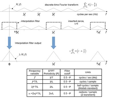
Let $X(f)$ be the Fourier transform of any function, $x(t),$ whose samples at some interval, $T,$ equal the $x[n]$ sequence. Then the discrete-time Fourier transform (DTFT) of the $x[n]$ sequence is the Fourier series representation of a periodic summation of $X(f):$Template:Efn-la

When $T$ has units of seconds, $f$ has units of hertz (Hz). Sampling $L$ times faster (at interval $T/L$) increases the periodicity by a factor of $L:$Template:Efn-la

which is also the desired result of interpolation. An example of both these distributions is depicted in the first and third graphs of Fig 2. 

When the additional samples are inserted zeros, they decrease the sample-interval to $T/L.$ Omitting the zero-valued terms of the Fourier series, it can be written as:

$\sum _{n=0,\pm L,\pm 2L,...,\pm \mathrm{\infty }}x(nT/L)e^{-i2\pi fnT/L}\stackrel{m\triangleq n/L}{⟶}\sum _{m=0,\pm 1,\pm 2,...,\pm \mathrm{\infty }}x(mT)e^{-i2\pi fmT},$

which is equivalent to Template:EquationNote regardless of the value of $L.$ That equivalence is depicted in the second graph of Fig.2. The only difference is that the available digital bandwidth is expanded to $L/T$, which increases the number of periodic spectral images within the new bandwidth. Some authors describe that as new frequency components.  The second graph also depicts a lowpass filter and $L=3,$ resulting in the desired spectral distribution (third graph). The filter's bandwidth is the Nyquist frequency of the original $x[n]$ sequence.Template:Efn-ua  In units of Hz that value is $\frac{0.5}{T},$  but filter design applications usually require normalized units. (see Fig 2, table)

Upsampling by a fractional factor

Let L/M denote the upsampling factor, where L > M.

1. Upsample by a factor of L
2. Downsample by a factor of M

Upsampling requires a lowpass filter after increasing the data rate, and downsampling requires a lowpass filter before decimation. Therefore, both operations can be accomplished by a single filter with the lower of the two cutoff frequencies. For the L > M case, the interpolation filter cutoff,  $\frac{0.5}{L}$ cycles per intermediate sample, is the lower frequency.

See also

• Downsampling
• Multi-rate digital signal processing
• Half-band filter
• Oversampling
• Sampling (information theory)
• Signal (information theory)
• Data conversion
• Interpolation
• Poisson summation formula

Further reading

• Template:Cite web (discusses a technique for bandlimited interpolation)
• Template:Cite web