Charge-pump phase-locked loop

Charge-pump PLL

Charge-pump phase-locked loop (CP-PLL) is a modification of phase-locked loops with phase-frequency detectors and square waveform signals. A CP-PLL allows for a quick lock of the phase of the incoming signal, achieving low steady state phase error.

Phase-frequency detector (PFD)

Phase-frequency detector dynamics

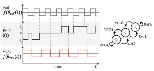
Phase-frequency detector (PFD) is triggered by the trailing edges of the reference (Ref) and controlled (VCO) signals. The output signal of PFD $i(t)$ can have only three states: 0, $+I_p$, and $-I_p$. A trailing edge of the reference signal forces the PFD to switch to a higher state, unless it is already in the state $+I_p$. A trailing edge of the VCO signal forces the PFD to switch to a lower state, unless it is already in the state $-I_p$. If both trailing edges happen at the same time, then the PFD switches to zero.

Mathematical models of CP-PLL

A first linear mathematical model of second-order CP-PLL was suggested by F. Gardner in 1980. A nonlinear model without the VCO overload was suggested by M. van Paemel in 1994 and then refined by N. Kuznetsov et al. in 2019. The closed form mathematical model of CP-PLL taking into account the VCO overload is derived in.

These mathematical models of CP-PLL allow to get analytical estimations of the hold-in range (a maximum range of the input signal period such that there exists a locked state at which the VCO is not overloaded) and the pull-in range (a maximum range of the input signal period within the hold-in range such that for any initial state the CP-PLL acquires a locked state).

Continuous time linear model of the second order CP-PLL and Gardner's conjecture

Gardner's analysis is based on the following approximation: time interval on which PFD has non-zero state on each period of reference signal is

$t_p=|{\theta }_e|/{\omega }_{\mathrm{r}\mathrm{e}\mathrm{f}},{\theta }_e={\theta }_{\mathrm{r}\mathrm{e}\mathrm{f}}-{\theta }_{\mathrm{v}\mathrm{c}\mathrm{o}}.$

Then averaged output of charge-pump PFD is

$i_d=I_p{\theta }_e/2\pi$

with corresponding transfer function

$I_d(s)=I_p{\theta }_e(s)/2\pi$

Using filter transfer function $F(s)=R+\frac{1}{Cs}$ and VCO transfer function ${\theta }_{\mathrm{v}\mathrm{c}\mathrm{o}}(s)=K_{\mathrm{v}\mathrm{c}\mathrm{o}}{I}_d(s)F(s)/s$ one gets Gardner's linear approximated average model of second-order CP-PLL

$\frac{{\theta }_e(s)}{{\theta }_{\mathrm{r}\mathrm{e}\mathrm{f}}(s)}=\frac{2\pi s}{2\pi s+K_{\mathrm{v}\mathrm{c}\mathrm{o}}{I}_p(R+\frac{1}{Cs})}.$

In 1980, F. Gardner, based on the above reasoning, conjectured that transient response of practical charge-pump PLL's can be expected to be nearly the same as the response of the equivalent classical PLLTemplate:Rp (Gardner's conjecture on CP-PLL). Following Gardner's results, by analogy with the Egan conjecture on the pull-in range of type 2 APLL, Amr M. Fahim conjectured in his bookTemplate:Rp that in order to have an infinite pull-in(capture) range, an active filter must be used for the loop filter in CP-PLL (Fahim-Egan's conjecture on the pull-in range of type II CP-PLL).

Continuous time nonlinear model of the second order CP-PLL

Without loss of generality it is supposed that trailing edges of the VCO and Ref signals occur when the corresponding phase reaches an integer number. Let the time instance of the first trailing edge of the Ref signal is defined as $t=0$. The PFD state $i(0)$ is determined by the PFD initial state $i(0-)$, the initial phase shifts of the VCO ${\theta }_{vco}(0)$ and Ref ${\theta }_{ref}(0)$ signals.

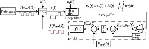
The relationship between the input current $i(t)$ and the output voltage $v_F(t)$ for a proportionally integrating (perfect PI) filter based on resistor and capacitor is as follows

$\begin{array}{c}{v}_F(t)=v_c(0)+Ri(t)+\frac{1}{C}\underset{0}{\overset{t}{\int }}i(\tau )d\tau \end{array}$

where $R>0$ is a resistance, $C>0$ is a capacitance, and $v_c(t)$ is a capacitor charge. The control signal $v_F(t)$ adjusts the VCO frequency:

$\begin{array}{c}{\dot{\theta }}_{vco}(t)={\omega }_{vco}(t)={\omega }_{vco}^{\text{free}}+K_{vco}{v}_F(t),\end{array}$

where ${\omega }_{vco}^{\text{free}}$ is the VCO free-running (quiescent) frequency (i.e. for $v_F(t)\equiv 0$), $K_{vco}$ is the VCO gain (sensivity), and ${\theta }_{vco}(t)$ is the VCO phase. Finally, the continuous time nonlinear mathematical model of CP-PLL is as follows

$\begin{array}{c}{\dot{v}}_c(t)=\frac{1}{C}i(t),{\dot{\theta }}_{vco}(t)={\omega }_{vco}^{\text{free}}+K_{vco}(Ri(t)+v_c(t))\end{array}$

with the following discontinuous piece-wise constant nonlinearity

$i(t)=i(i(t-),{\theta }_{ref}(t),{\theta }_{vco}(t))$

and the initial conditions $(v_c(0),{\theta }_{vco}(0))$. This model is a nonlinear, non-autonomous, discontinuous, switching system.

Discrete time nonlinear model of the second-order CP-PLL

Time intervals of the PFD dynamics

The reference signal frequency is assumed to be constant: ${\theta }_{ref}(t)={\omega }_{ref}t=\frac{t}{T_{ref}},$ where $T_{ref}$, ${\omega }_{ref}$ and ${\theta }_{ref}(t)$ are a period, frequency and a phase of the reference signal. Let $t_0=0$. Denote by $t_0^{\mathrm{m}\mathrm{i}\mathrm{d}\mathrm{d}\mathrm{l}\mathrm{e}}$ the first instant of time such that the PFD output becomes zero (if $i(0)=0$, then $t_0^{\mathrm{m}\mathrm{i}\mathrm{d}\mathrm{d}\mathrm{l}\mathrm{e}}=0$) and by $t_1$ the first trailing edge of the VCO or Ref. Further the corresponding increasing sequences $\{t_k\}$ and $\{t_k^{\mathrm{m}\mathrm{i}\mathrm{d}\mathrm{d}\mathrm{l}\mathrm{e}}\}$ for $k=0,1,2...$ are defined. Let $t_k<t_k^{\mathrm{m}\mathrm{i}\mathrm{d}\mathrm{d}\mathrm{l}\mathrm{e}}$. Then for $t\in [t_k,t_k^{\mathrm{m}\mathrm{i}\mathrm{d}\mathrm{d}\mathrm{l}\mathrm{e}})$ the $\text{sign}(i(t))$ is a non-zero constant ($\pm 1$). Denote by ${\tau }_k$ the PFD pulse width (length of the time interval, where the PFD output is a non-zero constant), multiplied by the sign of the PFD output: i.e. ${\tau }_k=(t_k^{\mathrm{m}\mathrm{i}\mathrm{d}\mathrm{d}\mathrm{l}\mathrm{e}}-t_k)\text{sign}(i(t))$ for $t\in [t_k,t_k^{\mathrm{m}\mathrm{i}\mathrm{d}\mathrm{d}\mathrm{l}\mathrm{e}})$ and ${\tau }_k=0$ for $t_k=t_k^{\mathrm{m}\mathrm{i}\mathrm{d}\mathrm{d}\mathrm{l}\mathrm{e}}$. If the VCO trailing edge hits before the Ref trailing edge, then ${\tau }_k<0$ and in the opposite case we have ${\tau }_k>0$, i.e. ${\tau }_k$ shows how one signal lags behind another. Zero output of PFD $i(t)\equiv 0$ on the interval $(t_k^{\mathrm{m}\mathrm{i}\mathrm{d}\mathrm{d}\mathrm{l}\mathrm{e}},t_{k+1})$: $v_F(t)\equiv v_k$ for $t\in [t_k^{\mathrm{m}\mathrm{i}\mathrm{d}\mathrm{d}\mathrm{l}\mathrm{e}},t_{k+1})$. The transformation of variables $({\tau }_k,v_k)$ to $p_k=\frac{{\tau }_k}{T_{\mathrm{r}\mathrm{e}\mathrm{f}}},u_k=T_{\mathrm{r}\mathrm{e}\mathrm{f}}({\omega }_{\mathrm{v}\mathrm{c}\mathrm{o}}^{\text{free}}+K_{\mathrm{v}\mathrm{c}\mathrm{o}}{v}_k)-1,$ allows to reduce the number of parameters to two: $\alpha =K_{\mathrm{v}\mathrm{c}\mathrm{o}}{I}_p{T}_{\mathrm{r}\mathrm{e}\mathrm{f}}R,\beta =\frac{K_{\mathrm{v}\mathrm{c}\mathrm{o}}{I}_p{T}_{\mathrm{r}\mathrm{e}\mathrm{f}}^2}{2C}.$ Here $p_k$ is a normalized phase shift and $u_k+1$ is a ratio of the VCO frequency ${\omega }_{\mathrm{v}\mathrm{c}\mathrm{o}}^{\text{free}}+K_{\mathrm{v}\mathrm{c}\mathrm{o}}{v}_k$ to the reference frequency $\frac{1}{T_{\mathrm{r}\mathrm{e}\mathrm{f}}}$. Finally, the discrete-time model of second order CP-PLL without the VCO overload

$\begin{array}{cc}& u_{k+1}=u_k+2\beta p_{k+1},\\ & p_{k+1}=\{\begin{array}{c}\frac{-(u_k+\alpha +1)+\sqrt{(u_k+\alpha +1{)}^2-4\beta c_k}}{2\beta },\text{ for }{p}_k\ge 0,c_k\le 0,\\ \frac{1}{u_k+1}-1+(p_k\text{ mod }1),\text{ for }{p}_k\ge 0,c_k>0,\\ l_k-1,\text{ for }{p}_k<0,l_k\le 1,\\ \frac{-(u_k+\alpha +1)+\sqrt{(u_k+\alpha +1{)}^2-4\beta d_k}}{2\beta },\text{ for }{p}_k<0,l_k>1,\end{array}\end{array}$

where

$\begin{array}{c}{c}_k=(1-(p_k\text{ mod }1))(u_k+1)-1,S_{l_k}=-(u_k-\alpha +1)p_k+\beta p_k^2,l_k=\frac{1-(S_{l_k}\text{ mod }1)}{u_k+1},d_k=(S_{l_k}\text{ mod }1)+u_k.\end{array}$

This discrete-time model has the only one steady state at $(u_k=0,p_k=0)$ and allows to estimate the hold-in and pull-in ranges.

If the VCO is overloaded, i.e. ${\dot{\theta }}_{\mathrm{v}\mathrm{c}\mathrm{o}}(t)$ is zero, or what is the same: $(p_k>0,u_k<2\beta p_k-1)$ or $(p_k<0,u_k<\alpha -1)$, then the additional cases of the CP-PLL dynamics have to be taken into account. For any parameters the VCO overload may occur for sufficiently large frequency difference between the VCO and reference signals. In practice the VCO overload should be avoided.

Nonlinear models of high-order CP-PLL

Derivation of nonlinear mathematical models of high-order CP-PLL leads to transcendental phase equations that cannot be solved analytically and require numerical approaches like the classical fixed-point method or the Newton-Raphson approach.