Faddeev–LeVerrier algorithm

Urbain Le Verrier (1811–1877)
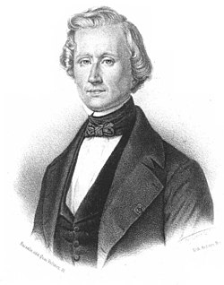
The discoverer of Neptune.

In mathematics (linear algebra), the Faddeev–LeVerrier algorithm is a recursive method to calculate the coefficients of the characteristic polynomial $p_A(\lambda )=\det (\lambda I_n-A)$ of a square matrix, Template:Mvar, named after Dmitry Konstantinovich Faddeev and Urbain Le Verrier. Calculation of this polynomial yields the eigenvalues of Template:Mvar as its roots; as a matrix polynomial in the matrix Template:Mvar itself, it vanishes by the Cayley–Hamilton theorem. Computing the characteristic polynomial directly from the definition of the determinant is computationally cumbersome insofar as it introduces a new symbolic quantity $\lambda$; by contrast, the Faddeev-Le Verrier algorithm works directly with coefficients of matrix $A$.

The algorithm has been independently rediscovered several times in different forms. It was first published in 1840 by Urbain Le Verrier, subsequently redeveloped by P. Horst, Jean-Marie Souriau, in its present form here by Faddeev and Sominsky, and further by J. S. Frame, and others. (For historical points, see Householder. An elegant shortcut to the proof, bypassing Newton polynomials, was introduced by Hou. The bulk of the presentation here follows Gantmacher, p. 88.)

The Algorithm

The objective is to calculate the coefficients Template:Math of the characteristic polynomial of the Template:Math matrix Template:Mvar,

$p_A(\lambda )\equiv \det (\lambda I_n-A)=\sum _{k=0}^n{c}_k{\lambda }^k,$

where, evidently, Template:Math = 1 and Template:Math₀ = (−1)ⁿ det Template:Mvar.

The coefficients Template:Math are determined by induction on Template:Mvar, using an auxiliary sequence of matrices

$\begin{array}{ccccc}{M}_0& \equiv 0& c_n& =1& (k=0)\\ M_k& \equiv A{M}_{k-1}+c_{n-k+1}I& c_{n-k}& =-\frac{1}{k}\mathrm{t}\mathrm{r}(A{M}_k)& k=1,\dots ,n.\end{array}$

Thus,

$M_1=I,c_{n-1}=-\mathrm{t}\mathrm{r}A=-c_n\mathrm{t}\mathrm{r}A;$

$M_2=A-I\mathrm{t}\mathrm{r}A,c_{n-2}=-\frac{1}{2}(\mathrm{t}\mathrm{r}{A}^2-(\mathrm{t}\mathrm{r}A{)}^2)=-\frac{1}{2}(c_n\mathrm{t}\mathrm{r}{A}^2+c_{n-1}\mathrm{t}\mathrm{r}A);$

$M_3=A^2-A\mathrm{t}\mathrm{r}A-\frac{1}{2}(\mathrm{t}\mathrm{r}{A}^2-(\mathrm{t}\mathrm{r}A{)}^2)I,$

$c_{n-3}=-\frac{1}{6}((\mathrm{tr}A{)}^3-3\mathrm{tr}(A^2)(\mathrm{tr}A)+2\mathrm{tr}(A^3))=-\frac{1}{3}(c_n\mathrm{t}\mathrm{r}{A}^3+c_{n-1}\mathrm{t}\mathrm{r}{A}^2+c_{n-2}\mathrm{t}\mathrm{r}A);$

etc.,   ...;

$M_m=\sum _{k=1}^m{c}_{n-m+k}{A}^{k-1},$

$c_{n-m}=-\frac{1}{m}(c_n\mathrm{t}\mathrm{r}{A}^m+c_{n-1}\mathrm{t}\mathrm{r}{A}^{m-1}+...+c_{n-m+1}\mathrm{t}\mathrm{r}A)=-\frac{1}{m}\sum _{k=1}^m{c}_{n-m+k}\mathrm{t}\mathrm{r}{A}^k;...$

Observe Template:Math terminates the recursion at Template:Mvar. This could be used to obtain the inverse or the determinant of Template:Mvar.

Derivation

The proof relies on the modes of the adjugate matrix, Template:Math, the auxiliary matrices encountered.   This matrix is defined by

$(\lambda I-A)B=I{p}_A(\lambda )$

and is thus proportional to the resolvent

$B=(\lambda I-A{)}^{-1}I{p}_A(\lambda ).$

It is evidently a matrix polynomial in Template:Math of degree Template:Math. Thus,

$B\equiv \sum _{k=0}^{n-1}{\lambda }^k{B}_k=\sum _{k=0}^n{\lambda }^k{M}_{n-k},$

where one may define the harmless Template:Math≡0.

Inserting the explicit polynomial forms into the defining equation for the adjugate, above,

$\sum _{k=0}^n{\lambda }^{k+1}{M}_{n-k}-{\lambda }^k(A{M}_{n-k}+c_{k}I)=0.$

Now, at the highest order, the first term vanishes by Template:Math=0; whereas at the bottom order (constant in Template:Mvar, from the defining equation of the adjugate, above),

$M_{n}A=B_{0}A=c_0,$

so that shifting the dummy indices of the first term yields

$\sum _{k=1}^n{\lambda }^k(M_{1+n-k}-A{M}_{n-k}+c_{k}I)=0,$

which thus dictates the recursion

$\therefore M_m=A{M}_{m-1}+c_{n-m+1}I,$

for Template:Mvar=1,...,Template:Mvar. Note that ascending index amounts to descending in powers of Template:Mvar, but the polynomial coefficients Template:Mvar are yet to be determined in terms of the Template:Mvars and Template:Mvar.

This can be easiest achieved through the following auxiliary equation (Hou, 1998),

$\lambda \frac{\partial p_A(\lambda )}{\partial \lambda }-np=\mathrm{tr}AB.$

This is but the trace of the defining equation for Template:Mvar by dint of Jacobi's formula,

$\frac{\partial p_A(\lambda )}{\partial \lambda }=p_A(\lambda )\sum _{m=0}^{\mathrm{\infty }}{\lambda }^{-(m+1)}\mathrm{tr}{A}^m=p_A(\lambda )\mathrm{tr}\frac{I}{\lambda I-A}\equiv \mathrm{tr}B.$

Inserting the polynomial mode forms in this auxiliary equation yields

$\sum _{k=1}^n{\lambda }^k(k{c}_k-n{c}_k-\mathrm{tr}A{M}_{n-k})=0,$

so that

$\sum _{m=1}^{n-1}{\lambda }^{n-m}(m{c}_{n-m}+\mathrm{tr}A{M}_m)=0,$

and finally

$\therefore c_{n-m}=-\frac{1}{m}\mathrm{tr}A{M}_m.$

This completes the recursion of the previous section, unfolding in descending powers of Template:Mvar.

Further note in the algorithm that, more directly,

$M_m=A{M}_{m-1}-\frac{1}{m-1}(\mathrm{tr}A{M}_{m-1})I,$

and, in comportance with the Cayley–Hamilton theorem,

$\mathrm{adj}(A)=(-1{)}^{n-1}{M}_n=(-1{)}^{n-1}(A^{n-1}+c_{n-1}{A}^{n-2}+...+c_{2}A+c_{1}I)=(-1{)}^{n-1}\sum _{k=1}^n{c}_k{A}^{k-1}.$

The final solution might be more conveniently expressed in terms of complete exponential Bell polynomials as

$c_{n-k}=\frac{(-1{)}^{n-k}}{k!}{ℬ}_k(\mathrm{tr}A,-1!\mathrm{tr}{A}^2,2!\mathrm{tr}{A}^3,\dots ,(-1{)}^{k-1}(k-1)!\mathrm{tr}{A}^k).$

Example

$A=\left[\begin{array}{ccc}3& 1& 5\\ 3& 3& 1\\ 4& 6& 4\end{array}\right]$

$\begin{array}{ccccccccccc}{M}_0& =\left[\begin{array}{ccc}0& 0& 0\\ 0& 0& 0\\ 0& 0& 0\end{array}\right]& & & c_3& & & & & =& 1\\ M_{\mathrm{𝟏}}& =\left[\begin{array}{ccc}1& 0& 0\\ 0& 1& 0\\ 0& 0& 1\end{array}\right]& A{M}_1& =\left[\begin{array}{ccc}\mathrm{𝟑}& 1& 5\\ 3& \mathrm{𝟑}& 1\\ 4& 6& \mathrm{𝟒}\end{array}\right]& c_2& & & =-\frac{1}{\mathrm{𝟏}}\mathrm{𝟏}\mathrm{𝟎}& & =& -10\\ M_{\mathrm{𝟐}}& =\left[\begin{array}{ccc}-7& 1& 5\\ 3& -7& 1\\ 4& 6& -6\end{array}\right]& A{M}_2& =\left[\begin{array}{ccc}\mathrm{𝟐}& 26& -14\\ -8& \mathbf{-}\mathrm{𝟏}\mathrm{𝟐}& 12\\ 6& -14& \mathrm{𝟐}\end{array}\right]& c_1& & & =-\frac{1}{\mathrm{𝟐}}\mathbf{(}\mathbf{-}\mathrm{𝟖}\mathbf{)}& & =& 4\\ M_{\mathrm{𝟑}}& =\left[\begin{array}{ccc}6& 26& -14\\ -8& -8& 12\\ 6& -14& 6\end{array}\right]& A{M}_3& =\left[\begin{array}{ccc}\mathrm{𝟒}\mathrm{𝟎}& 0& 0\\ 0& \mathrm{𝟒}\mathrm{𝟎}& 0\\ 0& 0& \mathrm{𝟒}\mathrm{𝟎}\end{array}\right]& c_0& & & =-\frac{1}{\mathrm{𝟑}}\mathrm{𝟏}\mathrm{𝟐}\mathrm{𝟎}& & =& -40\end{array}$

Furthermore, $M_4=A{M}_3+c_{0}I=0$, which confirms the above calculations.

The characteristic polynomial of matrix Template:Mvar is thus $p_A(\lambda )={\lambda }^3-10{\lambda }^2+4\lambda -40$; the determinant of Template:Mvar is $\det (A)=(-1{)}^3{c}_0=40$; the trace is 10=−c₂; and the inverse of Template:Mvar is

$A^{-1}=-\frac{1}{c_0}{M}_3=\frac{1}{40}\left[\begin{array}{ccc}6& 26& -14\\ -8& -8& 12\\ 6& -14& 6\end{array}\right]=\left[\begin{array}{ccc}0.15& 0.65& -0.35\\ -0.20& -0.20& 0.30\\ 0.15& -0.35& 0.15\end{array}\right]$.

An equivalent but distinct expression

A compact determinant of an Template:Mvar×Template:Mvar-matrix solution for the above Jacobi's formula may alternatively determine the coefficients Template:Mvar,

$c_{n-m}=\frac{(-1{)}^m}{m!}\left|\begin{array}{ccccc}\mathrm{tr}A& m-1& 0& \cdots & 0\\ \mathrm{tr}{A}^2& \mathrm{tr}A& m-2& \cdots & 0\\ ⋮& ⋮& & & ⋮\\ \mathrm{tr}{A}^{m-1}& \mathrm{tr}{A}^{m-2}& \cdots & \cdots & 1\\ \mathrm{tr}{A}^m& \mathrm{tr}{A}^{m-1}& \cdots & \cdots & \mathrm{tr}A\end{array}\right|.$

See also

• Characteristic polynomial
• Horner's method
• Fredholm determinant

References

Template:Reflist Barbaresco F. (2019) Souriau Exponential Map Algorithm for Machine Learning on Matrix Lie Groups. In: Nielsen F., Barbaresco F. (eds) Geometric Science of Information. GSI 2019. Lecture Notes in Computer Science, vol 11712. Springer, Cham. https://doi.org/10.1007/978-3-030-26980-7_10