Coordinate descent

Template:Short description Coordinate descent is an optimization algorithm that successively minimizes along coordinate directions to find the minimum of a function. At each iteration, the algorithm determines a coordinate or coordinate block via a coordinate selection rule, then exactly or inexactly minimizes over the corresponding coordinate hyperplane while fixing all other coordinates or coordinate blocks. A line search along the coordinate direction can be performed at the current iterate to determine the appropriate step size. Coordinate descent is applicable in both differentiable and derivative-free contexts.

Description

Coordinate descent is based on the idea that the minimization of a multivariable function $F(𝐱)$ can be achieved by minimizing it along one direction at a time, i.e., solving univariate (or at least much simpler) optimization problems in a loop. In the simplest case of cyclic coordinate descent, one cyclically iterates through the directions, one at a time, minimizing the objective function with respect to each coordinate direction at a time. That is, starting with initial variable values

${𝐱}^0=(x_1^0,\dots ,x_n^0)$,

round $k+1$ defines ${𝐱}^{k+1}$ from ${𝐱}^k$ by iteratively solving the single variable optimization problems

$x_i^{k+1}=\underset{y\in ℝ}{\mathrm{a}\mathrm{r}\mathrm{g}\mathrm{m}\mathrm{i}\mathrm{n}}f(x_1^{k+1},\dots ,x_{i-1}^{k+1},y,x_{i+1}^k,\dots ,x_n^k)$

for each variable $x_i$ of $𝐱$, for $i$ from 1 to $n$.

Thus, one begins with an initial guess ${𝐱}^0$ for a local minimum of $F$, and gets a sequence ${𝐱}^0,{𝐱}^1,{𝐱}^2,\dots$ iteratively.

By doing line search in each iteration, one automatically has

$F({𝐱}^0)\ge F({𝐱}^1)\ge F({𝐱}^2)\ge \dots .$

It can be shown that this sequence has similar convergence properties as steepest descent. No improvement after one cycle of line search along coordinate directions implies a stationary point is reached.

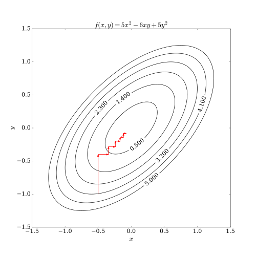
This process is illustrated below.

Differentiable case

In the case of a continuously differentiable function Template:Mvar, a coordinate descent algorithm can be sketched as:Template:R

• Choose an initial parameter vector Template:Math.
• Until convergence is reached, or for some fixed number of iterations:
  • Choose an index Template:Mvar from Template:Math to Template:Mvar.
  • Choose a step size Template:Mvar.
  • Update Template:Mvar to Template:Math.

The step size can be chosen in various ways, e.g., by solving for the exact minimizer of Template:Math (i.e., Template:Mvar with all variables but Template:Mvar fixed), or by traditional line search criteria.Template:R

Limitations

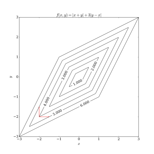
Coordinate descent has two problems. One of them is the case of a non-smooth objective function. The following picture shows that coordinate descent iteration may get stuck at a non-stationary point if the level curves of the function are not smooth. Suppose that the algorithm is at the point Template:Math; then there are two axis-aligned directions it can consider for taking a step, indicated by the red arrows. However, every step along these two directions will increase the objective function's value (assuming a minimization problem), so the algorithm will not take any step, even though both steps together would bring the algorithm closer to the optimum. While this example shows that coordinate descent does not necessarily converge to the optimum, it is possible to show formal convergence under reasonable conditions.

The other problem is difficulty in parallelism. Since the nature of coordinate descent is to cycle through the directions and minimize the objective function with respect to each coordinate direction, coordinate descent is not an obvious candidate for massive parallelism. Recent research works have shown that massive parallelism is applicable to coordinate descent by relaxing the change of the objective function with respect to each coordinate direction.

Applications

Coordinate descent algorithms are popular with practitioners owing to their simplicity, but the same property has led optimization researchers to largely ignore them in favor of more interesting (complicated) methods.Template:R An early application of coordinate descent optimization was in the area of computed tomography where it has been found to have rapid convergence and was subsequently used for clinical multi-slice helical scan CT reconstruction. A cyclic coordinate descent algorithm (CCD) has been applied in protein structure prediction. Moreover, there has been increased interest in the use of coordinate descent with the advent of large-scale problems in machine learning, where coordinate descent has been shown competitive to other methods when applied to such problems as training linear support vector machines (see LIBLINEAR) and non-negative matrix factorization. They are attractive for problems where computing gradients is infeasible, perhaps because the data required to do so are distributed across computer networks.

See also

• Template:Annotated link
• Template:Annotated link
• Template:Annotated link
• Template:Annotated link
• Template:Annotated link
• Template:Annotated link
• Template:Annotated link – uses one example at a time, rather than one coordinate

References

• Template:Citation
• Bertsekas, Dimitri P. (1999). Nonlinear Programming, Second Edition Athena Scientific, Belmont, Massachusetts. Template:ISBN.
• Template:Citation.
• Template:Citation.
• Template:Citation.
• Template:Citation.