Method of steepest descent

Template:Short description Template:For In mathematics, the method of steepest descent or saddle-point method is an extension of Laplace's method for approximating an integral, where one deforms a contour integral in the complex plane to pass near a stationary point (saddle point), in roughly the direction of steepest descent or stationary phase. The saddle-point approximation is used with integrals in the complex plane, whereas Laplace’s method is used with real integrals.

The integral to be estimated is often of the form

$\underset{C}{\int }f(z)e^{\lambda g(z)}dz,$

where C is a contour, and λ is large. One version of the method of steepest descent deforms the contour of integration C into a new path integration C′ so that the following conditions hold:

1. C′ passes through one or more zeros of the derivative g′(z),
2. the imaginary part of g(z) is constant on C′.

The method of steepest descent was first published by Template:Harvtxt, who used it to estimate Bessel functions and pointed out that it occurred in the unpublished note by Template:Harvtxt about hypergeometric functions. The contour of steepest descent has a minimax property, see Template:Harvtxt. Template:Harvtxt described some other unpublished notes of Riemann, where he used this method to derive the Riemann–Siegel formula.

Basic idea

The method of steepest descent is a method to approximate a complex integral of the form$$I(\lambda )=\underset{C}{\int }f(z)e^{\lambda g(z)}\mathrm{d}z$$for large $\lambda \to \mathrm{\infty }$, where $f(z)$ and $g(z)$ are analytic functions of $z$. Because the integrand is analytic, the contour $C$ can be deformed into a new contour $C^{\prime }$ without changing the integral. In particular, one seeks a new contour on which the imaginary part, denoted $\mathrm{\Im }(\cdot )$, of $g(z)=\mathrm{\Re }[g(z)]+i\mathrm{\Im }[g(z)]$ is constant ($\mathrm{\Re }(\cdot )$ denotes the real part). Then $$I(\lambda )=e^{i\lambda \mathrm{\Im }\{g(z)\}}\underset{C^{\prime }}{\int }f(z)e^{\lambda \mathrm{\Re }\{g(z)\}}\mathrm{d}z,$$and the remaining integral can be approximated with other methods like Laplace's method.

Etymology

The method is called the method of steepest descent because for analytic $g(z)$, constant phase contours are equivalent to steepest descent contours.

If $g(z)=X(z)+iY(z)$ is an analytic function of $z=x+iy$, it satisfies the Cauchy–Riemann equations$$\frac{\partial X}{\partial x}=\frac{\partial Y}{\partial y}\text{and}\frac{\partial X}{\partial y}=-\frac{\partial Y}{\partial x}.$$Then $$\frac{\partial X}{\partial x}\frac{\partial Y}{\partial x}+\frac{\partial X}{\partial y}\frac{\partial Y}{\partial y}=\mathrm{\nabla }X\cdot \mathrm{\nabla }Y=0,$$so contours of constant phase are also contours of steepest descent.

A simple estimate

Let Template:Math and Template:Math. If

$M=\underset{x\in C}{\sup }\mathrm{\Re }(S(x))<\mathrm{\infty },$

where $\mathrm{\Re }(\cdot )$ denotes the real part, and there exists a positive real number Template:Math such that

$\underset{C}{\int }|f(x)e^{{\lambda }_{0}S(x)}|dx<\mathrm{\infty },$

then the following estimate holds:

$|\underset{C}{\int }f(x)e^{\lambda S(x)}dx|⩽\text{const}\cdot e^{\lambda M},\mathrm{\forall }\lambda \in ℝ,\lambda ⩾{\lambda }_0.$

Proof of the simple estimate:

$\begin{array}{cc}|\underset{C}{\int }f(x)e^{\lambda S(x)}dx|& ⩽\underset{C}{\int }|f(x)|\left|e^{\lambda S(x)}\right|dx\\ & \equiv \underset{C}{\int }|f(x)|e^{\lambda M}\left|e^{{\lambda }_0(S(x)-M)}{e}^{(\lambda -{\lambda }_0)(S(x)-M)}\right|dx\\ & ⩽\underset{C}{\int }|f(x)|e^{\lambda M}\left|e^{{\lambda }_0(S(x)-M)}\right|dx& & \left|e^{(\lambda -{\lambda }_0)(S(x)-M)}\right|⩽1\\ & =\underset{\text{const}}{\underbrace{e^{-{\lambda }_{0}M}\underset{C}{\int }|f(x)e^{{\lambda }_{0}S(x)}|dx}}\cdot e^{\lambda M}.\end{array}$

The case of a single non-degenerate saddle point

Basic notions and notation

Let Template:Mvar be a complex Template:Mvar-dimensional vector, and

$S^{\prime }{\text{'}}_{xx}(x)\equiv \left(\frac{{\partial }^{2}S(x)}{\partial x_i\partial x_j}\right),1⩽i,j⩽n,$

denote the Hessian matrix for a function Template:Math. If

$\mathit{\phi }(x)=({\phi }_1(x),{\phi }_2(x),\dots ,{\phi }_k(x))$

is a vector function, then its Jacobian matrix is defined as

${{\mathit{\phi }}_x}^{\prime }(x)\equiv \left(\frac{\partial {\phi }_i(x)}{\partial x_j}\right),1⩽i⩽k,1⩽j⩽n.$

A non-degenerate saddle point, Template:Math, of a holomorphic function Template:Math is a critical point of the function (i.e., Template:Math) where the function's Hessian matrix has a non-vanishing determinant (i.e., $\det S^{\prime }{\text{'}}_{zz}(z^0)\ne 0$).

The following is the main tool for constructing the asymptotics of integrals in the case of a non-degenerate saddle point:

Complex Morse lemma

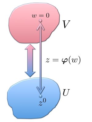
The Morse lemma for real-valued functions generalizes as follows for holomorphic functions: near a non-degenerate saddle point Template:Math of a holomorphic function Template:Math, there exist coordinates in terms of which Template:Math is exactly quadratic. To make this precise, let Template:Mvar be a holomorphic function with domain Template:Math, and let Template:Math in Template:Mvar be a non-degenerate saddle point of Template:Mvar, that is, Template:Math and $\det S^{\prime }{\text{'}}_{zz}(z^0)\ne 0$. Then there exist neighborhoods Template:Math of Template:Math and Template:Math of Template:Math, and a bijective holomorphic function Template:Math with Template:Math such that

$\mathrm{\forall }w\in V:S(\mathit{\phi }(w))=S(z^0)+\frac{1}{2}\sum _{j=1}^n{\mu }_j{w}_j^2,\det {{\mathit{\phi }}_w}^{\prime }(0)=1,$

Here, the Template:Math are the eigenvalues of the matrix $S_{z^{″}z}(z^0)$.

An illustration of Complex Morse lemma

The asymptotic expansion in the case of a single non-degenerate saddle point

Assume

1. Template:Math and Template:Math are holomorphic functions in an open, bounded, and simply connected set Template:Math such that the Template:Math is connected;
2. $\mathrm{\Re }(S(z))$ has a single maximum: $\underset{z\in I_x}{\max }\mathrm{\Re }(S(z))=\mathrm{\Re }(S(x^0))$ for exactly one point Template:Math;
3. Template:Math is a non-degenerate saddle point (i.e., Template:Math and $\det S^{\prime }{\text{'}}_{xx}(x^0)\ne 0$).

Then, the following asymptotic holds Template:NumBlk where Template:Math are eigenvalues of the Hessian $S^{\prime }{\text{'}}_{xx}(x^0)$ and $(-{\mu }_j{)}^{-\frac{1}{2}}$ are defined with arguments Template:NumBlk

This statement is a special case of more general results presented in Fedoryuk (1987). Template:Math proof

Equation (8) can also be written as

where the branch of

$\sqrt{\det (-S_{x^{″}x}(x^0))}$

is selected as follows

$\begin{array}{cc}{(\det (-S_{x^{″}x}(x^0)))}^{-\frac{1}{2}}& =\exp (-i\text{ Ind}(-S_{x^{″}x}(x^0)))\prod _{j=1}^n{\left|{\mu }_j\right|}^{-\frac{1}{2}},\\ \text{Ind}(-S_{x^{″}x}(x^0))& =\frac{1}{2}\sum _{j=1}^n\arg (-{\mu }_j),& & |\arg (-{\mu }_j)|<\frac{\pi }{2}.\end{array}$

Consider important special cases:

• If Template:Math is real valued for real Template:Mvar and Template:Math in Template:Math (aka, the multidimensional Laplace method), then $$\text{Ind}(-S_{x^{″}x}(x^0))=0.$$
• If Template:Math is purely imaginary for real Template:Mvar (i.e., $\mathrm{\Re }(S(x))=0$ for all Template:Mvar in Template:Math) and Template:Math in Template:Math (aka, the multidimensional stationary phase method), then $$\text{Ind}(-S_{x^{″}x}(x^0))=\frac{\pi }{4}\text{sign }{S}_{x^{″}x}(x_0),$$ where $\text{sign }{S}_{x^{″}x}(x_0)$ denotes the signature of matrix $S_{x^{″}x}(x_0)$, which equals to the number of negative eigenvalues minus the number of positive ones. It is noteworthy that in applications of the stationary phase method to the multidimensional WKB approximation in quantum mechanics (as well as in optics), Template:Math is related to the Maslov index see, e.g., Template:Harvtxt and Template:Harvtxt.

The case of multiple non-degenerate saddle points

If the function Template:Math has multiple isolated non-degenerate saddle points, i.e.,

$\mathrm{\nabla }S\left(x^{(k)}\right)=0,\det S^{\prime }{\text{'}}_{xx}\left(x^{(k)}\right)\ne 0,x^{(k)}\in {\mathrm{\Omega }}_x^{(k)},$

where

${\left\{{\mathrm{\Omega }}_x^{(k)}\right\}}_{k=1}^K$

is an open cover of Template:Math, then the calculation of the integral asymptotic is reduced to the case of a single saddle point by employing the partition of unity. The partition of unity allows us to construct a set of continuous functions Template:Math such that

$\begin{array}{cccc}\sum _{k=1}^K{\rho }_k(x)& =1,& & \mathrm{\forall }x\in {\mathrm{\Omega }}_x,\\ {\rho }_k(x)& =0& & \mathrm{\forall }x\in {\mathrm{\Omega }}_x\setminus {\mathrm{\Omega }}_x^{(k)}.\end{array}$

Whence,

$\underset{I_x\subset {\mathrm{\Omega }}_x}{\int }f(x)e^{\lambda S(x)}dx\equiv \sum _{k=1}^K\underset{I_x\subset {\mathrm{\Omega }}_x}{\int }{\rho }_k(x)f(x)e^{\lambda S(x)}dx.$

Therefore as Template:Math we have:

$\sum _{k=1}^K\underset{\text{a neighborhood of }{x}^{(k)}}{\int }f(x)e^{\lambda S(x)}dx={\left(\frac{2\pi }{\lambda }\right)}^{\frac{n}{2}}\sum _{k=1}^K{e}^{\lambda S\left(x^{(k)}\right)}{(\det (-S_{x^{″}x}\left(x^{(k)}\right)))}^{-\frac{1}{2}}f\left(x^{(k)}\right),$

where equation (13) was utilized at the last stage, and the pre-exponential function Template:Math at least must be continuous.

The other cases

When Template:Math and $\det S^{\prime }{\text{'}}_{zz}(z^0)=0$, the point Template:Math is called a degenerate saddle point of a function Template:Math.

Calculating the asymptotic of

$\int f(x)e^{\lambda S(x)}dx,$

when Template:Math is continuous, and Template:Math has a degenerate saddle point, is a very rich problem, whose solution heavily relies on the catastrophe theory. Here, the catastrophe theory replaces the Morse lemma, valid only in the non-degenerate case, to transform the function Template:Math into one of the multitude of canonical representations. For further details see, e.g., Template:Harvtxt and Template:Harvtxt.

Integrals with degenerate saddle points naturally appear in many applications including optical caustics and the multidimensional WKB approximation in quantum mechanics.

The other cases such as, e.g., Template:Math and/or Template:Math are discontinuous or when an extremum of Template:Math lies at the integration region's boundary, require special care (see, e.g., Template:Harvtxt and Template:Harvtxt).

Extensions and generalizations

An extension of the steepest descent method is the so-called nonlinear stationary phase/steepest descent method. Here, instead of integrals, one needs to evaluate asymptotically solutions of Riemann–Hilbert factorization problems.

Given a contour C in the complex sphere, a function f defined on that contour and a special point, say infinity, one seeks a function M holomorphic away from the contour C, with prescribed jump across C, and with a given normalization at infinity. If f and hence M are matrices rather than scalars this is a problem that in general does not admit an explicit solution.

An asymptotic evaluation is then possible along the lines of the linear stationary phase/steepest descent method. The idea is to reduce asymptotically the solution of the given Riemann–Hilbert problem to that of a simpler, explicitly solvable, Riemann–Hilbert problem. Cauchy's theorem is used to justify deformations of the jump contour.

The nonlinear stationary phase was introduced by Deift and Zhou in 1993, based on earlier work of the Russian mathematician Alexander Its. A (properly speaking) nonlinear steepest descent method was introduced by Kamvissis, K. McLaughlin and P. Miller in 2003, based on previous work of Lax, Levermore, Deift, Venakides and Zhou. As in the linear case, steepest descent contours solve a min-max problem. In the nonlinear case they turn out to be "S-curves" (defined in a different context back in the 80s by Stahl, Gonchar and Rakhmanov).

The nonlinear stationary phase/steepest descent method has applications to the theory of soliton equations and integrable models, random matrices and combinatorics.

Another extension is the Method of Chester–Friedman–Ursell for coalescing saddle points and uniform asymptotic extensions.

See also

• Pearcey integral
• Stationary phase approximation
• Laplace's method

References

• Template:Citation
• Template:Citation English translation in Template:Citation
• Template:Citation.
• Template:Citation.
• Template:Eom.
• Template:Citation [in Russian].
• Template:Citation.
• Template:Citation (Unpublished note, reproduced in Riemann's collected papers.)
• Template:Citation Reprinted in Gesammelte Abhandlungen, Vol. 1. Berlin: Springer-Verlag, 1966.
  • Translated in Template:Cite arXiv.
• Template:Citation.
• Template:Citation
• Template:Citation.