Algebraic connectivity

An example graph, with 6 vertices, diameter 3, connectivity 1, and algebraic connectivity 0.722

The algebraic connectivity (also known as Fiedler value or Fiedler eigenvalue after Miroslav Fiedler) of a graph Template:Mvar is the second-smallest eigenvalue (counting multiple eigenvalues separately) of the Laplacian matrix of Template:Mvar. This eigenvalue is greater than 0 if and only if Template:Mvar is a connected graph. This is a corollary to the fact that the number of times 0 appears as an eigenvalue in the Laplacian is the number of connected components in the graph. The magnitude of this value reflects how well connected the overall graph is. It has been used in analyzing the robustness and synchronizability of networks.

Properties

The truncated icosahedron or Buckminsterfullerene graph has a traditional connectivity of 3, and an algebraic connectivity of 0.243.

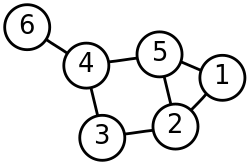
The algebraic connectivity of undirected graphs with nonnegative weights is $a(G)\ge 0$, with the inequality being strict if and only if Template:Mvar is connected. However, the algebraic connectivity can be negative for general directed graphs, even if Template:Mvar is a connected graph. Furthermore, the value of the algebraic connectivity is bounded above by the traditional (vertex) connectivity of a graph, $\text{algebraic connectivity}\le \text{connectivity}$, unless the graph is complete (the algebraic connectivity of a complete graph Template:Mvar is its order Template:Mvar). For an undirected connected graph with nonnegative edge weights, Template:Mvar vertices, and diameter Template:Mvar, the algebraic connectivity is also known to be bounded below by $\frac{1}{nD}$, and in fact (in a result due to Brendan McKay) by $\frac{4}{nD}$. For the example graph with 6 nodes show above ($n=6,D=3$), these bounds would be calculated as:$$4/18=0.222\le \text{algebraic connectivity 0.722}\le \text{connectivity 1.}$$Unlike the traditional form of graph connectivity, defined by local configurations whose removal would disconnect the graph, the algebraic connectivity is dependent on the global number of vertices, as well as the way in which vertices are connected. In random graphs, the algebraic connectivity decreases with the number of vertices, and increases with the average degree.

The exact definition of the algebraic connectivity depends on the type of Laplacian used. Fan Chung has developed an extensive theory using a rescaled version of the Laplacian, eliminating the dependence on the number of vertices, so that the bounds are somewhat different.

In models of synchronization on networks, such as the Kuramoto model, the Laplacian matrix arises naturally, so the algebraic connectivity gives an indication of how easily the network will synchronize. Other measures, such as the average distance (characteristic path length) can also be used, and in fact the algebraic connectivity is closely related to the (reciprocal of the) average distance.

The algebraic connectivity also relates to other connectivity attributes, such as the isoperimetric number, which is bounded below by half the algebraic connectivity.

Fiedler vector

The original theory related to algebraic connectivity was produced by Miroslav Fiedler. In his honor the eigenvector associated with the algebraic connectivity has been named the Fiedler vector. The Fiedler vector can be used to partition a graph.

Partitioning a graph using the Fiedler vector

Partitioning into two connected graphs

For the example graph in the introductory section, the Fiedler vector is $\left(\begin{array}{cccccc}0.415& 0.309& 0.069& -0.221& 0.221& -0.794\end{array}\right)$. The negative values are associated with the poorly connected vertex 6, and the neighbouring articulation point, vertex 4; while the positive values are associated with the other vertices. The signs of the values in the Fiedler vector can therefore be used to partition this graph into two components: $\{1,2,3,5\},\{4,6\}$. Alternatively, the value of 0.069 (which is close to zero) can be placed in a class of its own, partitioning the graph into three components: $\{1,2,5\},\{3\},\{4,6\}$ or moved to the other partition $\{1,2,5\},\{3,4,6\}$, as pictured. The squared values of the components of the Fiedler vector, summing up to one since the vector is normalized, can be interpreted as probabilities of the corresponding data points to be assigned to the sign-based partition.

See also

• Connectivity (graph theory)
• Graph property