Convexity in economics

Template:Short description Template:JEL code Template:Economics sidebar Convexity is a geometric property with a variety of applications in economics. Informally, an economic phenomenon is convex when "intermediates (or combinations) are better than extremes". For example, an economic agent with convex preferences prefers combinations of goods over having a lot of any one sort of good; this represents a kind of diminishing marginal utility of having more of the same good.

Convexity is a key simplifying assumption in many economic models, as it leads to market behavior that is easy to understand and which has desirable properties. For example, the Arrow–Debreu model of general economic equilibrium posits that if preferences are convex and there is perfect competition, then aggregate supplies will equal aggregate demands for every commodity in the economy.

In contrast, non-convexity is associated with market failures, where supply and demand differ or where market equilibria can be inefficient.

The branch of mathematics which supplies the tools for convex functions and their properties is called convex analysis; non-convex phenomena are studied under nonsmooth analysis.

Preliminaries

Template:Off topic The economics depends upon the following definitions and results from convex geometry.

Real vector spaces

A real vector space of two dimensions may be given a Cartesian coordinate system in which every point is identified by a list of two real numbers, called "coordinates", which are conventionally denoted by x and y. Two points in the Cartesian plane can be added coordinate-wise

(x₁, y₁) + (x₂, y₂) = (x₁+x₂, y₁+y₂);

further, a point can be multiplied by each real number λ coordinate-wise

λ (x, y) = (λx, λy).

More generally, any real vector space of (finite) dimension D can be viewed as the set of all possible lists of D real numbers Template:Nowrap } together with two operations: vector addition and multiplication by a real number. For finite-dimensional vector spaces, the operations of vector addition and real-number multiplication can each be defined coordinate-wise, following the example of the Cartesian plane.

Convex sets

In the convex hull of the red set, each blue point is a convex combination of some red points.

In a real vector space, a set is defined to be convex if, for each pair of its points, every point on the line segment that joins them is covered by the set. For example, a solid cube is convex; however, anything that is hollow or dented, for example, a crescent shape, is non‑convex. Trivially, the empty set is convex.

More formally, a set Q is convex if, for all points v₀ and v₁ in Q and for every real number λ in the unit interval Template:Closed-closed, the point

(1 − λ) v₀ + λv₁

is a member of Q.

By mathematical induction, a set Q is convex if and only if every convex combination of members of Q also belongs to Q. By definition, a convex combination of an indexed subset {v₀, v₁, . . . , v_D} of a vector space is any weighted average Template:Nowrap for some indexed set of non‑negative real numbers {λ_d} satisfying the equation Template:Nowrap = 1.

The definition of a convex set implies that the intersection of two convex sets is a convex set. More generally, the intersection of a family of convex sets is a convex set.

Convex hull

For every subset Q of a real vector space, its Template:Nowrap is the minimal convex set that contains Q. Thus Conv(Q) is the intersection of all the convex sets that cover Q. The convex hull of a set can be equivalently defined to be the set of all convex combinations of points in Q.

Duality: Intersecting half-spaces

A convex set $S$ (in pink), a supporting hyperplane of $S$ (the dashed line), and the half-space delimited by the hyperplane that contains $S$ (in light blue).

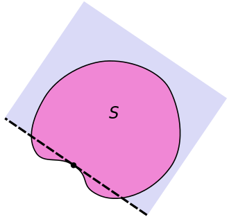
Supporting hyperplane is a concept in geometry. A hyperplane divides a space into two half-spaces. A hyperplane is said to support a set $S$ in the real n-space ${ℝ}^n$ if it meets both of the following:

• $S$ is entirely contained in one of the two closed half-spaces determined by the hyperplane
• $S$ has at least one point on the hyperplane.

Here, a closed half-space is the half-space that includes the hyperplane.

Supporting hyperplane theorem

A convex set can have more than one supporting hyperplane at a given point on its boundary.

This theorem states that if $S$ is a closed convex set in ${ℝ}^n,$ and $x$ is a point on the boundary of $S,$ then there exists a supporting hyperplane containing $x.$

The hyperplane in the theorem may not be unique, as noticed in the second picture on the right. If the closed set $S$ is not convex, the statement of the theorem is not true at all points on the boundary of $S,$ as illustrated in the third picture on the right.

A supporting hyperplane containing a given point on the boundary of $S$ may not exist if $S$ is not convex.

Economics

The consumer prefers the vector of goods (Q_x, Q_y) over other affordable vectors. At this optimal vector, the budget line supports the indifference curve I₂.

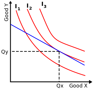
An optimal basket of goods occurs where the consumer's convex preference set is supported by the budget constraint, as shown in the diagram. If the preference set is convex, then the consumer's set of optimal decisions is a convex set, for example, a unique optimal basket (or even a line segment of optimal baskets).

For simplicity, we shall assume that the preferences of a consumer can be described by a utility function that is a continuous function, which implies that the preference sets are closed. (The meanings of "closed set" is explained below, in the subsection on optimization applications.)

Non-convexity

When consumer preferences have concavities, then the linear budgets need not support equilibria: Consumers can jump between allocations.

If a preference set is non‑convex, then some prices produce a budget supporting two different optimal consumption decisions. For example, we can imagine that, for zoos, a lion costs as much as an eagle, and further that a zoo's budget suffices for one eagle or one lion. We can suppose also that a zoo-keeper views either animal as equally valuable. In this case, the zoo would purchase either one lion or one eagle. Of course, a contemporary zoo-keeper does not want to purchase a half an eagle and a Template:Nowrap (or a griffin)! Thus, the contemporary zoo-keeper's preferences are non‑convex: The zoo-keeper prefers having either animal to having any strictly convex combination of both.

Non‑convex sets have been incorporated in the theories of general economic equilibria, of market failures, and of public economics. These results are described in graduate-level textbooks in microeconomics, general equilibrium theory, game theory, mathematical economics, and applied mathematics (for economists). The Shapley–Folkman lemma results establish that non‑convexities are compatible with approximate equilibria in markets with many consumers; these results also apply to production economies with many small firms.

In "oligopolies" (markets dominated by a few producers), especially in "monopolies" (markets dominated by one producer), non‑convexities remain important. Concerns with large producers exploiting market power in fact initiated the literature on non‑convex sets, when Piero Sraffa wrote about on firms with increasing returns to scale in 1926, after which Harold Hotelling wrote about marginal cost pricing in 1938. Both Sraffa and Hotelling illuminated the market power of producers without competitors, clearly stimulating a literature on the supply-side of the economy. Non‑convex sets arise also with environmental goods (and other externalities), with information economics, and with stock markets (and other incomplete markets). Such applications continued to motivate economists to study non‑convex sets.

Nonsmooth analysis

Template:Cleanup Economists have increasingly studied non‑convex sets with nonsmooth analysis, which generalizes convex analysis. "Non‑convexities in [both] production and consumption ... required mathematical tools that went beyond convexity, and further development had to await the invention of non‑smooth calculus" (for example, Francis Clarke's locally Lipschitz calculus), as described by Template:Harvtxt and Template:Harvtxt, according to Template:Harvtxt. Template:Harvtxt wrote that the "major methodological innovation in the general equilibrium analysis of firms with pricing rules" was "the introduction of the methods of non‑smooth analysis, as a [synthesis] of global analysis (differential topology) and [of] convex analysis." According to Template:Harvtxt, "Non‑smooth analysis extends the local approximation of manifolds by tangent planes [and extends] the analogous approximation of convex sets by tangent cones to sets" that can be non‑smooth or non‑convex. Economists have also used algebraic topology.

See also

• Convex duality

References

• Template:Cite book
• Template:Cite book
• Template:Cite book
• Template:Cite book
• Template:Cite book
• Template:Cite book
• Luenberger, David G. Microeconomic Theory, McGraw-Hill, Inc., New York, 1995.
• Template:Cite book
• Template:Cite book
• Template:Cite book
• Template:Cite book.
• Template:Cite book